AI review — page 7

claude-opus-4-8 · prompt v7 · 2026-08-21T10:44:45+00:00 · applied: yes · changed: yes

Screenshot sent to the model (reading-order tags burned on)

Instructions (system prompt)

The screenshot has annotations burned onto it that are NOT part of the document:
- a small red numbered tag at the top-left corner of each item, showing that item's position in the OCR-determined reading order (the same order the items appear in the json data);
- a red-and-white dotted outline around each item, showing the area the OCR detected for that content block.
Use the tags and outlines to see the detected reading order and item boundaries directly on the page, and judge that sequence against how a human would naturally read it. Ignore the annotations when checking text fidelity — they overlay the content, they are not content.

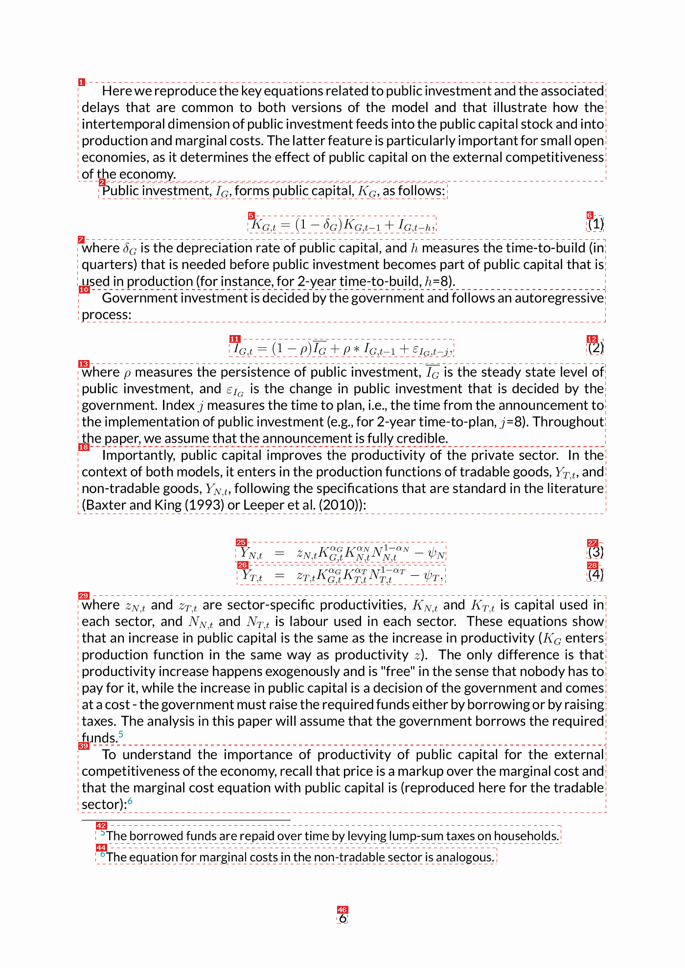
For the given screenshot of a PDF's page and the attached json data, I want you to perform the following tasks in order...

Review the reading order set out in the json data and compare to what a natural reading order for that of a human would be by looking at the screenshot. Decide on any changes and re-arrange the items for the most logical reading order.
Look at all text for each item and correct any extraction errors like missing words, spelling mistakes etc.
Look at each item in the JSON and ensure that the OCR process has identified the item as the correct type: text, list item etc.
Look for any text that duplicates: if two items next to each other contain the exact same text but the text only appears once on the screenshot, one of them is an extraction error — keep the item whose box matches where the text is visible and flag the other for removal.
Make amendments as you proceed through the items and list of instructions.
Reading Order Advice: If there is columns with headings and text, I wouldnt expect the reading order to jump from one heading straight to another if there is text associated with that heading.

Return format: Give me the json data back only, with the amendments you make.

Mechanical notes (so your answer can be applied automatically):
- Each item has an `id` — keep every item and its `id` exactly as given; never invent, drop or duplicate ids. Re-arranging means changing the position of items (and their nesting) in the arrays.
- Never move text (or a type) from one item to another: each item's coordinates travel with its id, so to change reading order you must move the whole item object, and text amendments must be in-place corrections of that item's own text.
- To flag a duplicate item, keep it in the array and add `"remove": "duplicate"` to it — never just delete it (deleted items are restored automatically).
- ids are opaque labels, not sequence numbers: never renumber them. After a removal or re-arrangement, every remaining item keeps the exact id it came with, even if the ids no longer look sequential.
- Text may contain `[pN.M…]` placeholders marking where an inline formula belongs — treat them as part of the text and leave them exactly where they are.
- `box` is [left, top, right, bottom] as percentages of the page from the top-left corner; return it unchanged.
- Respond with raw JSON only: no code fences, no commentary, same shape as the input (`{"items": [...]}`).

User message (json data sent)

Page 7 json data:

{"items":[{"id":"p7.1","type":"text","box":[11,8,88,19],"text":"Here we reproduce the key equations related to public investment and the associated delays that are common to both versions of the model and that illustrate how the intertemporal dimension of public investment feeds into the public capital stock and into production and marginal costs. The latter feature is particularly important for small open economies, as it determines the effect of public capital on the external competitiveness of the economy."},{"id":"p7.2","type":"text","box":[14,19,65,21],"text":"Public investment,[p7.2.1], forms public capital,[p7.2.2], as follows:","children":[{"id":"p7.2.1","type":"formula","box":[14,19,65,21],"text":"I_{G}"},{"id":"p7.2.2","type":"formula","box":[14,19,65,21],"text":"K_{G}"}]},{"id":"p7.3","type":"formula","box":[36,22,64,24],"text":"K_{G,t}=(1-\\delta_{G})K_{G,t-1}+I_{G,t-h},"},{"id":"p7.4","type":"text","box":[86,22,88,24],"text":"(1)"},{"id":"p7.5","type":"text","box":[11,25,88,30],"text":"where[p7.5.1] is the depreciation rate of public capital, and $h$ measures the time-to-build (in quarters) that is needed before public investment becomes part of public capital that is used in production (for instance, for 2-year time-to-build,[p7.5.2]).","children":[{"id":"p7.5.1","type":"formula","box":[11,25,88,30],"text":"\\delta_{G}"},{"id":"p7.5.2","type":"formula","box":[11,25,88,30],"text":"h = 8"}]},{"id":"p7.6","type":"text","box":[11,30,88,33],"text":"Government investment is decided by the government and follows an autoregressive process:"},{"id":"p7.7","type":"formula","box":[33,35,66,37],"text":"I_{G,t}=(1-\\rho)\\overline{{I_{G}}}+\\rho*I_{G,t-1}+\\varepsilon_{I_{G},t-j},"},{"id":"p7.8","type":"text","box":[86,35,88,37],"text":"(2)"},{"id":"p7.9","type":"text","box":[11,38,88,46],"text":"where[p7.9.1] measures the persistence of public investment,[p7.9.2] is the steady state level of public investment, and[p7.9.3] is the change in public investment that is decided by the government. Index $j$ measures the time to plan, i.e., the time from the announcement to the implementation of public investment (e.g., for 2-year time-to-plan,[p7.9.4]). Throughout the paper, we assume that the announcement is fully credible.","children":[{"id":"p7.9.1","type":"formula","box":[11,38,88,46],"text":"ρ"},{"id":"p7.9.2","type":"formula","box":[11,38,88,46],"text":"\\overline{I_{G}}"},{"id":"p7.9.3","type":"formula","box":[11,38,88,46],"text":"\\varepsilon_{I_{G}}"},{"id":"p7.9.4","type":"formula","box":[11,38,88,46],"text":"j = 8"}]},{"id":"p7.10","type":"text","box":[11,46,88,53],"text":"Importantly, public capital improves the productivity of the private sector. In the context of both models, it enters in the production functions of tradable goods,[p7.10.5], and non-tradable goods,[p7.10.6], following the specifications that are standard in the literature (Baxter and King (1993) or Leeper et al. (2010)):","children":[{"id":"p7.10.1","type":"link","box":[12,51,27,53],"text":"(Baxter and King"},{"id":"p7.10.2","type":"link","box":[27,51,32,53],"text":"(1993)"},{"id":"p7.10.3","type":"link","box":[35,51,46,53],"text":"Leeper et al."},{"id":"p7.10.4","type":"link","box":[47,51,52,53],"text":"(2010)):"},{"id":"p7.10.5","type":"formula","box":[11,46,88,53],"text":"Y_{T,t}"},{"id":"p7.10.6","type":"formula","box":[11,46,88,53],"text":"Y_{N,t}"}]},{"id":"p7.11","type":"formula","box":[34,56,65,58],"text":"\\begin{array}{ccl}{Y_{N,t}}&{=}&{z_{N,t}K_{G,t}^{\\alpha_{G}}K_{N,t}^{\\alpha_{N}}N_{N,t}^{1-\\alpha_{N}}-\\psi_{N}}\\\\ \\end{array}"},{"id":"p7.12","type":"formula","box":[35,58,65,60],"text":"\\begin{array}{lcl}{Y_{T,t}}&{=}&{z_{T,t}K_{G,t}^{\\alpha_{G}}K_{T,t}^{\\alpha_{T}}N_{T,t}^{1-\\alpha_{T}}-\\psi_{T},}\\\\ \\end{array}"},{"id":"p7.13","type":"text","box":[86,56,88,58],"text":"(3)"},{"id":"p7.14","type":"text","box":[86,58,88,60],"text":"(4)"},{"id":"p7.15","type":"text","box":[11,62,88,77],"text":"where[p7.15.2] and[p7.15.3] are sector-specific productivities,[p7.15.4] and[p7.15.5] is capital used in each sector, and[p7.15.6] and[p7.15.7] is labour used in each sector. These equations show that an increase in public capital is the same as the increase in productivity ([p7.15.8] enters production function in the same way as productivity z). The only difference is that productivity increase happens exogenously and is \"free\" in the sense that nobody has to pay for it, while the increase in public capital is a decision of the government and comes at a cost - the government must raise the required funds either by borrowing or by raising taxes. The analysis in this paper will assume that the government borrows the required funds. [p7.15.9]","children":[{"id":"p7.15.1","type":"link","box":[17,75,18,77],"text":"5"},{"id":"p7.15.2","type":"formula","box":[11,62,88,77],"text":"z_{N,t}"},{"id":"p7.15.3","type":"formula","box":[11,62,88,77],"text":"z_{T,t}"},{"id":"p7.15.4","type":"formula","box":[11,62,88,77],"text":"K_{N,t}"},{"id":"p7.15.5","type":"formula","box":[11,62,88,77],"text":"K_{T,t}"},{"id":"p7.15.6","type":"formula","box":[11,62,88,77],"text":"N_{N,t}"},{"id":"p7.15.7","type":"formula","box":[11,62,88,77],"text":"N_{T,t}"},{"id":"p7.15.8","type":"formula","box":[11,62,88,77],"text":"K_{G}"},{"id":"p7.15.9","type":"formula","box":[11,62,88,77],"text":"⁵"}]},{"id":"p7.16","type":"text","box":[11,77,88,84],"text":"To understand the importance of productivity of public capital for the external competitiveness of the economy, recall that price is a markup over the marginal cost and that the marginal cost equation with public capital is (reproduced here for the tradable sector): [p7.16.2]","children":[{"id":"p7.16.1","type":"link","box":[18,82,20,84],"text":"6"},{"id":"p7.16.2","type":"formula","box":[11,77,88,84],"text":"⁶"}]},{"id":"p7.17","type":"footnote","box":[14,85,82,87],"text":"[p7.17.1]The borrowed funds are repaid over time by levying lump-sum taxes on households.","children":[{"id":"p7.17.1","type":"formula","box":[14,85,82,87],"text":"⁵"}]},{"id":"p7.18","type":"footnote","box":[14,88,73,89],"text":"[p7.18.1]The equation for marginal costs in the non-tradable sector is analogous.","children":[{"id":"p7.18.1","type":"formula","box":[14,88,73,89],"text":"⁶"}]},{"id":"p7.19","type":"footer","box":[49,94,51,95],"text":"6"}]}